Differential Expression Analysis of the ALL Chiaretti Microarray Dataset with pylimma

This tutorial walks through a pre-normalised microarray workflow. The expression matrix arrives RMA-normalised, so voom is skipped; the analysis goes straight from the matrix to lm_fit.

R-parity validation: the sibling notebook `all_R_vs_Python.ipynb <all_R_vs_Python.ipynb>`__ runs R limma 3.66.0 on the same input and compares the outputs numerically.

Dataset

Chiaretti et al. 2004, Blood 103:2771-2778: Acute Lymphoblastic Leukemia gene-expression profiles from 128 patients on Affymetrix HG-U95Av2 arrays. The shipped matrix is the 12,625-probe RMA-normalised expression set from the BioBase::ALL Bioconductor package.

Biological question: B-cell (B) vs T-cell (T) derived leukemia cases.

Pipeline

1. Load expression matrix + phenotype targets

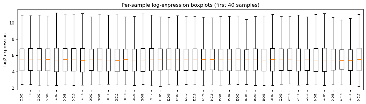
2. Per-sample distribution QC (boxplot)

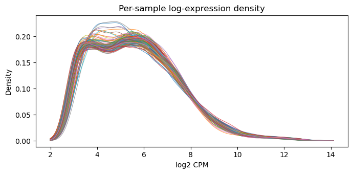
3. log-expression kernel density (sanity check)

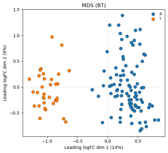
4. MDS (coloured by BT)

5. Design matrix

6. lm_fit + contrasts_fit

7. Empirical Bayes moderation

8. Top table and DE calling

9. MD + volcano plots

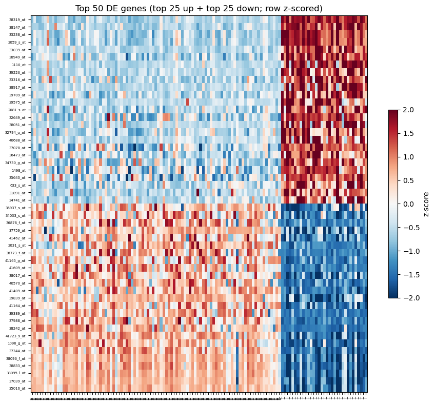
10. Heatmap of top 50 DE probes (row-ordered by signed t)

11. Summary

import sys
from pathlib import Path

import matplotlib.pyplot as plt
import numpy as np
import pandas as pd

REPO = Path.cwd().resolve().parents[1]
sys.path.insert(0, str(REPO))
sys.path.insert(0, str(REPO / 'data'))

import generate_data as gd

import pylimma

pd.set_option('display.width', 120)
pd.set_option('display.max_columns', 10)

# Shared plotting helpers used by every tutorial.

def _log_cpm(mat, lib_size):
    cpm = mat.div(lib_size, axis=1) * 1e6 if hasattr(mat, 'div') \
          else (mat / lib_size) * 1e6
    return np.log2(cpm + 1e-2)


def plot_log_cpm_density(mat, ax, title=""):
    '''Kernel-smoothed log-CPM density, one line per sample.

    Matches edgeR/limma's standard density plot (limma User's Guide
    Figure 15.1): a Gaussian KDE per sample drawn on a shared grid.
    '''
    from scipy.stats import gaussian_kde
    arr = mat.values if hasattr(mat, 'values') else np.asarray(mat)
    # Shared evaluation grid spanning the combined range.
    lo, hi = np.nanmin(arr), np.nanmax(arr)
    grid = np.linspace(lo, hi, 200)
    for j in range(arr.shape[1]):
        col = arr[:, j]
        col = col[np.isfinite(col)]
        if col.size < 2:
            continue
        kde = gaussian_kde(col)
        ax.plot(grid, kde(grid), linewidth=0.8, alpha=0.7)
    ax.set_xlabel('log2 CPM')
    ax.set_ylabel('Density')
    ax.set_title(title)


def mds_coords(mat, top=500):
    '''Pairwise leading-logFC MDS, matching R limma's plotMDS.default.

    Returns the (n_samples, ndim) coordinate matrix and the percent of
    variance explained per dimension. We reuse pylimma's private
    _mds_coordinates for consistency with plot_mds().
    '''
    from pylimma.plotting import _mds_coordinates
    r = _mds_coordinates(np.asarray(mat, dtype=np.float64), top=top,
                         gene_selection='pairwise', ndim=2)
    lam = np.maximum(r['eigen_values'], 0.0)
    coords = r['eigen_vectors'] * np.sqrt(lam)
    return coords, r['var_explained']


def plot_mds_coloured(mat, groups, ax, top=500, title='MDS'):
    '''MDS scatter plot coloured by sample group.'''
    coords, var_exp = mds_coords(mat, top=top)
    pct = np.round(var_exp * 100).astype(int)
    groups = np.asarray(groups)
    levels = sorted(pd.unique(groups))
    palette = plt.get_cmap('tab10').colors
    for k, level in enumerate(levels):
        m = groups == level
        ax.scatter(coords[m, 0], coords[m, 1],
                   s=55, color=palette[k % len(palette)],
                   label=str(level), edgecolor='k', linewidth=0.3)
    ax.axhline(0, color='grey', linewidth=0.4, linestyle=':')
    ax.axvline(0, color='grey', linewidth=0.4, linestyle=':')
    ax.set_xlabel(f'Leading logFC dim 1 ({pct[0]}%)')
    ax.set_ylabel(f'Leading logFC dim 2 ({pct[1]}%)')
    ax.set_title(title)
    ax.legend(fontsize=8, frameon=False)


def plot_heatmap(E, groups, fit, n_top=50, ax=None):
    '''Heatmap of top-n DE rows showing BOTH directions.

    Picks the top n/2 genes with the most positive t and the top n/2
    with the most negative t (by smallest p within each side), then
    stacks them - up-regulated in the contrast at top, down-regulated
    at bottom. Row z-scored.'''
    t = np.asarray(fit['t']).ravel()
    p = np.asarray(fit['p_value']).ravel()
    half = n_top // 2
    up_pool   = np.where(t > 0)[0]
    down_pool = np.where(t < 0)[0]
    top_up    = up_pool[np.argsort(p[up_pool])[:half]]
    top_down  = down_pool[np.argsort(p[down_pool])[:n_top - half]]
    # Sort each block by signed t descending so most-up is top and
    # most-down is bottom.
    top_up   = top_up[np.argsort(-t[top_up])]
    top_down = top_down[np.argsort(-t[top_down])]
    ordered  = np.concatenate([top_up, top_down])

    mat = E[ordered]
    col_order = np.argsort(groups)
    mat_sorted = mat[:, col_order]
    z = (mat_sorted - mat_sorted.mean(axis=1, keepdims=True)) / \
        (mat_sorted.std(axis=1, keepdims=True) + 1e-8)

    if ax is None:
        fig, ax = plt.subplots(figsize=(9, 8))
    im = ax.imshow(z, aspect='auto', cmap='RdBu_r', vmin=-2, vmax=2)
    ax.set_xticks(range(len(col_order)))
    ax.set_xticklabels(np.asarray(groups)[col_order], rotation=90, fontsize=6)
    ax.set_yticks([])
    ax.set_title(f'Top {n_top} DE genes (top {half} up + top {n_top - half} down; row z-scored)')
    return ax, im, ordered

1. Load the expression matrix + phenotype targets

data = gd.load_all()
expr    = data['expr']
targets = data['targets']
print(f"expression matrix: {expr.shape}  (probes x samples)")
group = targets["BT"].astype(str).str[0]
print("\nBT breakdown:")
print(group.value_counts())
targets[['BT', 'mol.biol', 'sex', 'age']].head()

expression matrix: (12625, 128)  (probes x samples)

BT breakdown:
BT
B    95
T    33
Name: count, dtype: int64

	BT	mol.biol	sex	age
01005	B2	BCR/ABL	M	53.0
01010	B2	NEG	M	19.0
03002	B4	BCR/ABL	F	52.0
04006	B1	ALL1/AF4	M	38.0
04007	B2	NEG	M	57.0

2. Per-sample distribution QC

fig, ax = plt.subplots(figsize=(12, 3.5))
ax.boxplot(expr.iloc[:, :40].values, labels=expr.columns[:40],
           showfliers=False)
ax.set_xticklabels(expr.columns[:40], rotation=90, fontsize=6)
ax.set_ylabel('log2 expression')
ax.set_title('Per-sample log-expression boxplots (first 40 samples)')
fig.tight_layout()
plt.show()

/var/folders/0x/4309q_jn5xbf3zzq_4hcp2100000gn/T/ipykernel_99358/2015273228.py:2: MatplotlibDeprecationWarning: The 'labels' parameter of boxplot() has been renamed 'tick_labels' since Matplotlib 3.9; support for the old name will be dropped in 3.11.
  ax.boxplot(expr.iloc[:, :40].values, labels=expr.columns[:40],

3. log-expression density (KDE)

Kernel density per sample. After RMA all samples should be nearly super-imposed - a visible outlier would warrant follow-up before differential analysis.

fig, ax = plt.subplots(figsize=(7, 3.5))
plot_log_cpm_density(expr, ax, 'Per-sample log-expression density')
fig.tight_layout()
plt.show()

4. MDS (coloured by BT)

fig, ax = plt.subplots(figsize=(5.5, 5))
plot_mds_coloured(expr.values, group.values, ax,
                  top=500, title='MDS (BT)')
fig.tight_layout()
plt.show()

5. Design matrix

design, C = gd.build_two_group_design(group)
design_df = pd.DataFrame(design, index=expr.columns,
                         columns=sorted(group.unique()))
print(f"Design: {design_df.shape}, contrast = T - B")
design_df.head(8)

Design: (128, 2), contrast = T - B

	B	T
01005	1.0	0.0
01010	1.0	0.0
03002	1.0	0.0
04006	1.0	0.0
04007	1.0	0.0
04008	1.0	0.0
04010	1.0	0.0
04016	1.0	0.0

6. Fit linear models and contrasts (no voom)

fit = pylimma.lm_fit(expr.values, design)
fit = pylimma.contrasts_fit(fit, contrasts=C)
print(f"coefficients shape: {fit['coefficients'].shape}")

/Users/John/miniconda3/lib/python3.11/site-packages/h5py/__init__.py:36: UserWarning: h5py is running against HDF5 1.14.3 when it was built against 1.14.2, this may cause problems
  _warn(("h5py is running against HDF5 {0} when it was built against {1}, "

coefficients shape: (12625, 1)

7. Empirical Bayes moderation

fit = pylimma.e_bayes(fit)
print(f"s2_prior: {fit['s2_prior']:.4f}")
print(f"df_prior: {fit['df_prior']:.2f}")

s2_prior: 0.0842
df_prior: 3.03

8. Top table

tt = pylimma.top_table(fit, coef=0, number=np.inf, sort_by='p')
tt.index = expr.index[np.argsort(np.asarray(fit['p_value']).ravel())]
print(f"DE calls at adj_p_value < 0.05: {(tt['adj_p_value'] < 0.05).sum():,} probes")
tt.head(10)

DE calls at adj_p_value < 0.05: 3,024 probes

	log_fc	ave_expr	t	p_value	adj_p_value	b
38319_at	4.655042	6.041217	35.302014	3.665982e-68	4.628303e-64	142.887385
38147_at	3.154743	4.582970	26.368452	8.329164e-54	5.257785e-50	111.276776
33238_at	3.102294	7.292159	22.711375	6.493588e-47	2.732718e-43	95.863304
35016_at	-3.214222	10.337892	-22.347402	3.433264e-46	1.083624e-42	94.239065
2059_s_at	2.668482	7.232735	22.156246	8.286073e-46	2.092233e-42	93.379248
37039_at	-3.265990	11.072596	-21.343275	3.694071e-44	7.772940e-41	89.669946
38095_i_at	-3.762299	10.228156	-20.426219	2.955978e-42	5.331317e-39	85.382469
38833_at	-2.966787	10.144085	-19.764032	7.473721e-41	1.179447e-37	82.217871
33039_at	1.812889	3.619621	19.685785	1.098739e-40	1.541287e-37	81.840104
38096_f_at	-4.248782	9.169628	-19.055233	2.522408e-39	3.184540e-36	78.766423

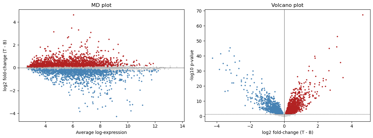
9. MD + volcano plots

logFC = fit['coefficients'][:, 0]
AveExpr = fit.get('Amean') if fit.get('Amean') is not None \
          else expr.mean(axis=1).values
adj_sig = pylimma.decide_tests(fit, p_value=0.05).ravel() != 0

fig, (axMD, axV) = plt.subplots(1, 2, figsize=(12, 4.5))
# MD
axMD.scatter(AveExpr[~adj_sig], logFC[~adj_sig], s=2, c='lightgrey')
axMD.scatter(AveExpr[adj_sig & (logFC > 0)],
             logFC[adj_sig & (logFC > 0)], s=4, c='firebrick')
axMD.scatter(AveExpr[adj_sig & (logFC < 0)],
             logFC[adj_sig & (logFC < 0)], s=4, c='steelblue')
axMD.axhline(0, color='k', linewidth=0.5)
axMD.set_xlabel('Average log-expression')
axMD.set_ylabel('log2 fold-change (T - B)')
axMD.set_title('MD plot')

# Volcano
p = np.asarray(fit['p_value']).ravel()
neglogp = -np.log10(np.maximum(p, 1e-300))
axV.scatter(logFC[~adj_sig], neglogp[~adj_sig], s=2, c='lightgrey')
axV.scatter(logFC[adj_sig & (logFC > 0)],
            neglogp[adj_sig & (logFC > 0)], s=4, c='firebrick')
axV.scatter(logFC[adj_sig & (logFC < 0)],
            neglogp[adj_sig & (logFC < 0)], s=4, c='steelblue')
axV.axhline(-np.log10(0.05), color='k', linewidth=0.5, linestyle='--')
axV.axvline(0, color='k', linewidth=0.5)
axV.set_xlabel('log2 fold-change (T - B)')
axV.set_ylabel('-log10 p-value')
axV.set_title('Volcano plot')
fig.tight_layout()
plt.show()

10. Heatmap of top 50 DE probes

Rows ordered by signed t-statistic (up-regulated at top, down-regulated at bottom). Columns grouped by BT.

fig, ax = plt.subplots(figsize=(9, 8))
ax, im, ordered = plot_heatmap(expr.values, group.values, fit,
                                n_top=50, ax=ax)
ax.set_yticks(range(len(ordered)))
ax.set_yticklabels(expr.index[ordered], fontsize=5)
fig.colorbar(im, ax=ax, shrink=0.5, label='z-score')
fig.tight_layout()
plt.show()