Differential abundance analysis of proteomics data with pylimma

This tutorial demonstrates the AnnData-native pylimma workflow on a bulk mass-spectrometry proteomics dataset. The matrix is already log-transformed and median-normalised, so the analysis is a classical microarray-style limma pipeline: build a design matrix, fit per-protein linear models, moderate variances with empirical Bayes, and read off the top differentially abundant proteins.

Dataset

Mulvey et al. 2026, Mol Cell Proteomics 25(2):101510. doi:10.1016/j.mcpro.2026.101510. Tissue proteomics from human left-ventricular tissue collected at heart transplantation or LVAD implantation (heart-failure cases) or from organ donors (controls). The original paper compares peripartum cardiomyopathy hearts against non-peripartum cardiomyopathy and controls; for this tutorial we collapse the two cardiomyopathy groups into a single heart_failure arm and contrast it against controls.

Shape: 7,026 protein groups x 15 samples (6 control donors + 9 heart-failure cases).

Pipeline

1. Load the protein abundance matrix and sample targets

2. Build an AnnData object (samples on obs, proteins on var)

3. PCA QC

4. Design matrix: ~ group

5. lm_fit -> e_bayes

6. Top differentially abundant proteins (heart-failure vs control)

7. Volcano plot

Loading the data

The two CSVs live under pylimma/data/ alongside the other bundled benchmark datasets (ALL, GSE60450, pasilla, Yoruba); see pylimma/data/DATA_PROVENANCE.md for the full provenance and licence summary.

import sys
import warnings
from pathlib import Path

import anndata as ad
import matplotlib.pyplot as plt
import numpy as np
import pandas as pd

warnings.filterwarnings('ignore', category=FutureWarning)

# This notebook lives at pylimma/pylimma/examples/mulvey/
# parents[1] = repo root (containing pylimma source + data/), matching
# the convention used by the other example notebooks.
REPO = Path.cwd().resolve().parents[1]
sys.path.insert(0, str(REPO))

import pylimma

DATA_DIR = REPO / 'data'
assert DATA_DIR.exists(), f'expected data dir at {DATA_DIR}'

pd.set_option('display.width', 120)
pd.set_option('display.max_columns', 12)

/Users/John/miniconda3/lib/python3.11/site-packages/h5py/__init__.py:36: UserWarning: h5py is running against HDF5 1.14.3 when it was built against 1.14.2, this may cause problems
  _warn(("h5py is running against HDF5 {0} when it was built against {1}, "

1. Load the matrix and targets

proteome = pd.read_csv(DATA_DIR / 'mulvey_proteome.csv.gz', index_col=0)
targets  = pd.read_csv(DATA_DIR / 'mulvey_targets.csv').set_index('sample_id')

protein_meta_cols = ['gene_symbol', 'num_psm',
                     'max_pep_prob', 'reference_intensity']
sample_cols       = [c for c in proteome.columns
                     if c not in protein_meta_cols]

X = proteome[sample_cols].T.values
var_df = proteome[protein_meta_cols].copy()
var_df.index.name = 'uniprot_id'

obs_df = targets.loc[sample_cols].copy()
obs_df['group'] = pd.Categorical(obs_df['group'],
                                  categories=['control', 'heart_failure'],
                                  ordered=False)

adata = ad.AnnData(X=X, obs=obs_df, var=var_df)
adata.obs_names = sample_cols
adata.var_names = var_df.index

print(f'AnnData shape: {adata.shape}  (samples x proteins)')
print(f'\ngroup counts:\n{adata.obs.group.value_counts()}')
adata.var.head()

AnnData shape: (15, 7026)  (samples x proteins)

group counts:
group
heart_failure    9
control          6
Name: count, dtype: int64

	gene_symbol	num_psm	max_pep_prob	reference_intensity
uniprot_id
A0A075B6H7	IGKV3-7	2	1.0000	16.264649
A0A075B6H9	IGLV4-69	2	1.0000	18.129858
A0A075B6I0	IGLV8-61	2	1.0000	18.895982
A0A075B6I1	IGLV4-60	3	1.0000	17.037598
A0A075B6I4	IGLV10-54	2	0.9998	15.915174

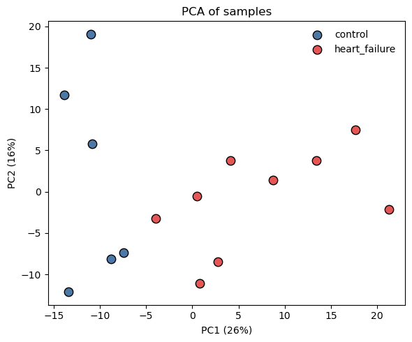
2. PCA QC

A PCA projection is a basic diagnostic to inspect before any DE analysis: separation between groups along an early PC indicates the contrast carries the expected signal.

fig, ax = plt.subplots(figsize=(6, 5))

# PCA on samples (centre proteins, drop any all-NaN rows just in case).
Xc = adata.X - adata.X.mean(axis=0, keepdims=True)
U, s, Vt = np.linalg.svd(Xc, full_matrices=False)
pcs = U * s
var_explained = (s ** 2) / (s ** 2).sum()

group_palette = {'control': '#4c78a8', 'heart_failure': '#e45756'}
for grp, colour in group_palette.items():
    m = (adata.obs['group'] == grp).values
    ax.scatter(pcs[m, 0], pcs[m, 1], s=80,
                color=colour, edgecolor='black', label=grp)
ax.set_xlabel(f'PC1 ({var_explained[0]:.0%})')
ax.set_ylabel(f'PC2 ({var_explained[1]:.0%})')
ax.set_title('PCA of samples')
ax.legend(frameon=False)

fig.tight_layout()
plt.show()

3. Design matrix and contrast

Two-level group factor with control as the reference level. The design has an intercept plus a heart_failure indicator; the contrast that asks “what is differentially abundant in heart failure versus control” is just the coefficient on the indicator (a one-element contrast vector [0, 1]).

group  = adata.obs['group']
design = pd.DataFrame({
    'Intercept':     1.0,
    'heart_failure': (group == 'heart_failure').astype(float).values,
}, index=adata.obs_names)

contrasts = pylimma.make_contrasts(HFvsCtrl='heart_failure', levels=design)

print('design matrix:')
print(design.head(3))
print('\ncontrast:')
print(contrasts)

design matrix:
       Intercept  heart_failure
Ctrl1        1.0            0.0
Ctrl2        1.0            0.0
Ctrl3        1.0            0.0

contrast:
               HFvsCtrl
Intercept           0.0
heart_failure       1.0

4. lm_fit -> contrasts_fit -> e_bayes

Pure AnnData pipeline. The fit is stored in adata.uns['pylimma'] and survives write_h5ad if you want to round-trip it through disk. No voom step here: the input is already log-scale normalised abundance, so we feed it straight into lm_fit.

pylimma.lm_fit(adata, design)
pylimma.contrasts_fit(adata, contrasts=contrasts)
pylimma.e_bayes(adata)

print('keys stored in adata.uns["pylimma"]:')
print(sorted(adata.uns['pylimma'].keys()))

keys stored in adata.uns["pylimma"]:
['Amean', 'F', 'F_p_value', 'coef_names', 'coefficients', 'contrast_names', 'contrasts', 'cov_coefficients', 'design', 'df_prior', 'df_residual', 'df_total', 'genes', 'lods', 'method', 'p_value', 'pivot', 'proportion', 'rank', 's2_post', 's2_prior', 'sigma', 'stdev_unscaled', 't', 'targets', 'var_prior']

5. Top differentially abundant proteins

top = pylimma.top_table(adata, coef='HFvsCtrl',
                         number=np.inf, sort_by='p')

# Carry over gene symbols from adata.var so the table is readable.
top = top.join(adata.var[['gene_symbol']], how='left')

n_sig_05 = int((top['adj_p_value'] < 0.05).sum())
n_sig_01 = int((top['adj_p_value'] < 0.01).sum())
print(f'differentially abundant proteins at adj_p_value < 0.05: {n_sig_05:,}')
print(f'differentially abundant proteins at adj_p_value < 0.01: {n_sig_01:,}')

display_cols = ['gene_symbol', 'log_fc', 'ave_expr', 't',
                'p_value', 'adj_p_value', 'b']
top.loc[:, display_cols].head(15).round(3)

differentially abundant proteins at adj_p_value < 0.05: 267
differentially abundant proteins at adj_p_value < 0.01: 0

	gene_symbol	log_fc	ave_expr	t	p_value	adj_p_value	b
gene
P02768	ALB	0.776	10.394	7.232	0.0	0.012	5.006
O43272	PRODH	-1.117	0.421	-6.932	0.0	0.012	4.550
Q9HDC5	JPH1	-0.522	-0.142	-6.422	0.0	0.015	3.738
Q9UBX5	FBLN5	1.266	2.883	6.364	0.0	0.015	3.644
P0DJI8	SAA1	-1.665	0.410	-6.290	0.0	0.015	3.522
Q8WTS1	ABHD5	-0.533	-0.134	-6.077	0.0	0.015	3.166
Q53HC5	KLHL26	0.466	-3.695	6.060	0.0	0.015	3.137
P31939	ATIC	-0.412	4.120	-6.045	0.0	0.015	3.112
Q6UX53	METTL7B	-0.867	0.794	-5.841	0.0	0.015	2.762
L0R8F8	MIEF1	-0.513	-1.684	-5.834	0.0	0.015	2.751
Q9H511	KLHL31	-0.392	1.800	-5.796	0.0	0.015	2.685
Q9UI14	RABAC1	-0.474	-1.084	-5.794	0.0	0.015	2.680
O60437	PPL	-0.678	0.905	-5.767	0.0	0.015	2.634
Q3ZCW2	LGALSL	0.448	-0.162	5.751	0.0	0.015	2.607
P05452	CLEC3B	0.809	1.326	5.477	0.0	0.022	2.123

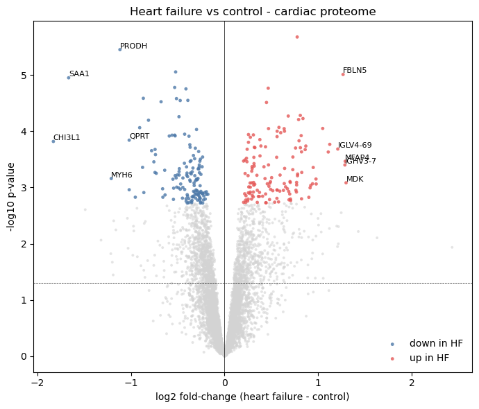
6. Volcano plot

Standard summary plot. Each point is one protein group; the x-axis is the log fold-change in heart failure relative to control, the y-axis is -log10(p_value). Proteins past adj_p_value < 0.05 are coloured red (up in heart failure) or blue (down in heart failure). Top hits by signed log fold-change are labelled with their gene symbol.

fig, ax = plt.subplots(figsize=(7, 6))

sig_up   = (top['adj_p_value'] < 0.05) & (top['log_fc'] > 0)
sig_down = (top['adj_p_value'] < 0.05) & (top['log_fc'] < 0)
ns       = ~(sig_up | sig_down)

nlp = -np.log10(np.maximum(top['p_value'].values, 1e-300))

ax.scatter(top.loc[ns, 'log_fc'],   nlp[ns.values],
           s=8, color='lightgrey', alpha=0.6, edgecolor='none')
ax.scatter(top.loc[sig_down, 'log_fc'], nlp[sig_down.values],
           s=12, color='#4c78a8', alpha=0.8,
           edgecolor='none', label='down in HF')
ax.scatter(top.loc[sig_up, 'log_fc'],   nlp[sig_up.values],
           s=12, color='#e45756', alpha=0.8,
           edgecolor='none', label='up in HF')

# Label the top 5 up and top 5 down by signed log fold change among the
# significant proteins (those past adj_p_value < 0.05). Gene symbols
# only - some entries have multi-gene proteingroup labels which we skip
# to keep the plot legible.
sig = top[top['adj_p_value'] < 0.05].copy()
top_up   = sig.sort_values('log_fc', ascending=False).head(5)
top_down = sig.sort_values('log_fc', ascending=True ).head(5)
for _, row in pd.concat([top_up, top_down]).iterrows():
    label = row['gene_symbol']
    if not isinstance(label, str) or ';' in label or label == '':
        continue
    ax.annotate(label, (row['log_fc'], -np.log10(max(row['p_value'], 1e-300))),
                fontsize=8, ha='left', va='bottom')

ax.axhline(-np.log10(0.05), color='black', lw=0.5, linestyle='--')
ax.axvline(0, color='black', lw=0.5)
ax.set_xlabel('log2 fold-change (heart failure - control)')
ax.set_ylabel('-log10 p-value')
ax.set_title('Heart failure vs control - cardiac proteome')
ax.legend(frameon=False, loc='lower right')
fig.tight_layout()
plt.show()